SPT Data Processing

© 2023 Daniel F. Ruiz, Exneyder A. Montoya-Araque y Universidad EAFIT.

This notebook can be interactively run in Google - Colab.

This notebook was developed following the procedure by Gonzalez [1999] for estimating the shear strength parameters from the Standard Penetration Test data (paper in Spanish).

Required modules and global setup for plots

import numpy as np
import pandas as pd
import matplotlib.pyplot as plt
import matplotlib as mpl
from scipy.optimize import curve_fit, minimize
from ipywidgets import widgets as wgt
from IPython import get_ipython
from IPython.display import display

if 'google.colab' in str(get_ipython()):
    print('Running on CoLab. Installing the required modules...')
    from subprocess import run
    # run('pip install ipympl', shell=True);
    from google.colab import output, files
    output.enable_custom_widget_manager()
else:
    import tkinter as tk
    from tkinter.filedialog import askopenfilename

# Figures setup
# %matplotlib widget
mpl.rcParams.update({
    "font.family": "serif",
    "font.serif": ["Computer Modern Roman", "cmr", "cmr10", "DejaVu Serif"],  # or 
    "mathtext.fontset": "cm",  # Use Computer Modern fonts for math
    "axes.formatter.use_mathtext": True,  # Use mathtext for axis labels
    "axes.unicode_minus": False,   # Use standard minus sign instead of a unicode character
})

Funciones

def x_from_y(x_coord, y_coord, target_y):
    for i in range(len(y_coord)):
        if y_coord[i] == target_y:  # if target_y coincides with a node
            if i < len(y_coord) and y_coord[i+1] == y_coord[i]:  # if on a horizontal segment:
                return 0.5 * (x_coord[i] + x_coord[i+1])  # return midpoint in x
            else:
                return x_coord[i]
        elif i > 0 and y_coord[i-1] < target_y < y_coord[i]:
            # Interpolate x-value when the target y-value lies between two points
            x1, x2 = x_coord[i-1], x_coord[i]
            y1, y2 = y_coord[i-1], y_coord[i]
            return x1 + (x2 - x1) * (target_y - y1) / (y2 - y1)
    return None  # Return None if y-value not found within the range

def compute_stresses(df, mat_depths, 𝛾_moist, 𝛾_sat, wt_depth=None):
    𝛾_w = 9.81  # unit weight of water [kN/m³]
    # Copying arrays
    mat_depths = mat_depths.copy()
    𝛾_moist = 𝛾_moist.copy()
    𝛾_sat = 𝛾_sat.copy()
    # Find an appropiate index for locating the watertable
    if wt_depth in mat_depths:
        idx_wt = mat_depths.index(wt_depth)
    elif wt_depth >= mat_depths[-1] or wt_depth is None:
        wt_depth = mat_depths[-1]
        idx_wt = len(mat_depths) - 1
    else:
        for i in range(len(mat_depths)):
            if wt_depth <= mat_depths[i]:
                idx_wt = i
                break
    # Insert the new value at the appropriate index
    mat_depths.insert(idx_wt, wt_depth)
    𝛾_moist.insert(idx_wt, 𝛾_moist[idx_wt])
    𝛾_sat.insert(idx_wt, 𝛾_sat[idx_wt])
    # Create an unified unit weight vector
    𝛾_s = 𝛾_moist[: idx_wt + 1] + 𝛾_sat[idx_wt + 1 :]
    # Create vector of thicknesses
    mat_depths.insert(0, 0)  # insert zero for the first layer
    thickness = np.diff(mat_depths)  # thickness of each soil layer [m]
    # Create a vector for unit weigth of water (zero above wt, and 𝛾_w below)
    𝛾_w = np.full_like(𝛾_s, 𝛾_w)
    𝛾_w[: idx_wt + 1] = 0
    # Compute vertical stresses and water pressure at boundaries
    𝜎_v = np.insert(np.cumsum(thickness * 𝛾_s), 0, 0)
    p_w = np.insert(np.cumsum(thickness * 𝛾_w), 0, 0)
    𝜎_v_eff = 𝜎_v - p_w
    df['Sigma_eff_(kPa)'] = [
        x_from_y(x_coord=𝜎_v_eff, y_coord=mat_depths, target_y=z)
        for z in df['Profundidad_(m)'].to_numpy()
    ]
    return

def compute_corrected_N(df, perfo_diam, field_test_energy):
    # Stress level correction
    n, 𝜎_ref = 0.5, 95.76  # reference stress level = 1 tsf(short) to kPa
    # df['Cn'] = (𝜎_ref / df['Sigma_eff_(kPa)']) ** n  # Liao y Whitman (1986)
    df['Cn'] = 2 / (1 + df['Sigma_eff_(kPa)']/𝜎_ref)  # Skempton (1986)
    # Correction factor to reach an standard energy level of 60%
    df['n1_E60'] = field_test_energy / 60
    # Correction factor due to the length of the drill rod
    n2 = np.empty_like(df['Profundidad_(m)'], dtype=float)
    depth = df['Profundidad_(m)'].to_numpy()
    n2[depth >= 10] = 1
    n2[depth < 10] = 0.95
    n2[depth < 6] = 0.85
    n2[depth < 4] = 0.75
    df['n2'] = n2
    # Correction factor due to the cassing
    mat_type = np.array([int(d[0]) for d in df['Descripción'].to_list()])
    n3 = np.ones_like(df['Profundidad_(m)'], dtype=float)
    n3[mat_type == 1] = 0.8
    n3[mat_type == 2] = 0.8
    n3[mat_type == 3] = 0.9
    n3[mat_type == 4] = 0.8
    n3[mat_type == 5] = 0.85
    n3[mat_type == 6] = 0.9
    n3[df['Revestimiento_(m)'] < df['Profundidad_(m)']] = 1
    df['n3'] = n3
    # Correction factor due to the hole diameter
    if perfo_diam <= 120:
        df['n4'] = 1
    elif perfo_diam <= 150:
        df['n4'] = 1.05
    elif perfo_diam > 150:
        df['n4'] = 1.15
    # N corrected
    df['N45'] = np.int64(df['N_campo'] * df['Cn'] * df['n2'] * df['n3'] * df['n4'] * field_test_energy / 45)
    df['N55'] = np.int64(df['N_campo'] * df['Cn'] * df['n2'] * df['n3'] * df['n4'] * field_test_energy / 55)
    df['N60'] = np.int64(df['N_campo'] * df['Cn'] * df['n2'] * df['n3'] * df['n4'] * field_test_energy / 60)

def compute_correlations(df, corr_𝜙='f'):
    '''
    Correlations for the friction angle based on the letters accompanying the
    formulas (7) and (8) in Gonzalez (1999)
    '''
    # Equivalent friction angle
    if corr_𝜙 == 'a':  # Peck
        df['𝜙_eq'] = 28.5 + 0.25 * df['N45']
    elif corr_𝜙 == 'b':  # Peck, Hanson & Thornburn
        df['𝜙_eq'] = 26.25 * (2 - np.exp(-1 * df['N45']/62))
    elif corr_𝜙 == 'c':  # Kishida
        df['𝜙_eq'] = 15 + (12.5 * df['N45']) ** 0.5
    elif corr_𝜙 == 'd':  # Schmertmann
        df['𝜙_eq'] = np.arctan((df['N45'] / 43.3)**0.34)
    elif corr_𝜙 == 'e':  # Japan National Railway (JNR)
        df['𝜙_eq'] = 27 + 0.1875 * df['N45']
    elif corr_𝜙 == 'f':  # Japan Road Bureau (JRB)
        df['𝜙_eq'] = 15 + (9.375 * df['N45']) ** 0.5
    # Equivalent shear strength 
    df['𝜏_eq'] = df['Sigma_eff_(kPa)'] * np.tan(np.deg2rad(df['𝜙_eq']))
    # Undrained shear strength based on Schmertmann (1975)
    df['Su_(kPa)'] = df['N60'] / 15 * 95.76
    # Put nan to 'Su_(kPa)' where fines are < 50% or isnan
    df.loc[df['Finos_(%)'] < 50, 'Su_(kPa)'] = np.nan
    df.loc[df['Finos_(%)'].isna(), 'Su_(kPa)'] = np.nan
    # Elasticity modulus
    mat_type = np.array([int(d[0]) for d in df['Descripción'].to_list()])
    elastic_mod = np.ones_like(df['Profundidad_(m)'])
    elastic_mod[mat_type == 1] = (250 * (df['N55'] + 15))[mat_type == 1]
    elastic_mod[mat_type == 2] = (500 * (df['N55'] + 15))[mat_type == 2]
    elastic_mod[mat_type == 3] = (40000 + (df['N55'] * 1050))[mat_type == 3]
    mask_4a = np.logical_and(mat_type == 4, df['N55'] <= 15)
    elastic_mod[mask_4a] = (600 * (df['N55'] + 6))[mask_4a]
    mask_4b = np.logical_and(mat_type == 4, df['N55'] > 15)
    elastic_mod[mask_4b] = (2000 + (600 * (df['N55'] + 6)))[mask_4b]
    elastic_mod[mat_type == 5] = (320 * (df['N55'] + 15))[mat_type == 5]
    elastic_mod[mat_type == 6] = (300 * (df['N55'] + 6))[mat_type == 6]
    df['Es_(kPa)'] = elastic_mod


def complete_table(df, mat_depths, 𝛾_moist, 𝛾_sat, wt_depth=None, perfo_diam=75,
                   field_test_energy=60, corr_𝜙='f'):
    compute_stresses(df, mat_depths, 𝛾_moist, 𝛾_sat, wt_depth)
    compute_corrected_N(df, perfo_diam, field_test_energy)
    compute_correlations(df, corr_𝜙='f')

def f_mc(x, m, b):  # Linear function for Mohr-Coulomb envelope with non-zero intercept
    return m * x + b

def f_mc_b0(x, m):  # Linear function for Mohr-Coulomb envelope with zero intercept forced if negative
    return m * x


palette = mpl.colors.ListedColormap(['#4477AA', '#EE6677', '#228833', '#CCBB44', '#66CCEE', '#AA3377', '#BBBBBB'])
palette = mpl.colors.ListedColormap(['#004488', '#DDAA33', '#BB5566', '#6699CC', '#EECC66', '#EE99AA'])


def plot_processing(df, mat_depths, wt_depth, plot_su=True, figsize=None):
    if figsize is None:
        figsize = [9, 6]
    fig, axs = plt.subplot_mosaic([['A', 'B', 'B'], ['A', '.', '.']],
                              layout='constrained', figsize=figsize)
    # Set Dark2 as the default color cycle
    # plt.style.use('seaborn-darkgrid')
    plt.rcParams.update({'axes.prop_cycle': plt.cycler(color=palette.colors)})

    # Create a twin axis for Su in axs['A'] if plot_su is True
    if plot_su:
        ax_twin = axs['B'].twinx()

    # Plotting the fine fraction content
    if 'Finos_(%)' in df.columns:
        if not df['Finos_(%)'].isna().all():  # check if it's not full of nan
            axs['A'].plot(df['Finos_(%)'], df['Profundidad_(m)'], ls="",
                        marker="|", mfc="w", mec="k", ms=10, mew=2.5, label="Fine fraction [%]")
    for i, mat in enumerate(df['Material'].unique()):
        df_mat = df[df['Material'] == mat]
        # Plotting N values vs depth
        axs['A'].plot(df_mat['N_campo'], df_mat['Profundidad_(m)'], ls="", marker="o", ms=6,
                      mfc=mpl.colors.to_rgba(f"C{i}", 0.8), mec=mpl.colors.to_rgba('k', 1), mew=.75)#, label=mat)
        # Plotting shear strength vs sigma_v
        axs['B'].plot(df_mat['Sigma_eff_(kPa)'], df_mat['𝜏_eq'], ls="", marker="o", ms=6,
                      mfc=mpl.colors.to_rgba(f"C{i}", 0.8), mec=mpl.colors.to_rgba('k', 1), mew=.75, label=mat)
        if len(df_mat) == 1:
            phi = df_mat['𝜙_eq'].values[0]
            m, b = np.tan(np.deg2rad(phi)), 0.0
            axs['B'].plot(df_mat['Sigma_eff_(kPa)'], m * df_mat['Sigma_eff_(kPa)'] + b,
                        ls=':', c=f"C{i}", label=f"$\\phi'={phi:.1f}^\\circ$")
        else:
            m, b = curve_fit(f_mc, df_mat['Sigma_eff_(kPa)'], df_mat['𝜏_eq'])[0]
            if b < 0:
                m, b = curve_fit(f_mc_b0, df_mat['Sigma_eff_(kPa)'], df_mat['𝜏_eq'])[0][0], 0.0
            # phi = np.rad2deg(m)
            phi = np.rad2deg(np.arctan(m))  # Correction by O. Perafán (2025/04/19)
            axs['B'].plot(df_mat['Sigma_eff_(kPa)'], m * df_mat['Sigma_eff_(kPa)'] + b,
                        ls=':', c=f"C{i}", label=f"$\\phi'={phi:.1f}^\\circ$, $c'={b:.1f}$ kPa")
        # Plotting Su values vs depth in a twin axis if plot_su is True
        if plot_su and not np.isnan(df_mat['Su_(kPa)'].mean()):
            label = f"Average $S_\\mathrm{{u}} = {df_mat['Su_(kPa)'].mean():.1f}$ kPa"
            ax_twin.plot(df_mat['Sigma_eff_(kPa)'], df_mat['Su_(kPa)'], ls="", marker="_", ms=7,
                         mec=mpl.colors.to_rgba(f"C{i}", 1), mew=2.5)#, label=label)
            # Fake plot in the original axis to show the legend
            axs['B'].plot([], [], ls="", marker="_", ms=7, mec=mpl.colors.to_rgba(f"C{i}", 1),
                          mew=2.5, label=label)
    for d in mat_depths:
        axs['A'].axhline(d, color="k", ls="--", lw=1.25)
    axs['A'].axhline(0, color="g", ls="-", lw=3.0, label="Terrain surface")
    axs['A'].axhline(np.nan, color="k", ls="--", lw=1.25, label="Material boundary")
    axs['A'].axhline(y=wt_depth, ls="-", color="XKCD:electric blue", lw=1.25, label="Watertable")

    # Plot setup
    axs['A'].invert_yaxis()
    # invert y-axis for depth for the twin axis
    if plot_su:
        ax_twin.set_ylabel("$S_\\mathrm{u}$  [kPa]")
        ax_twin.spines["right"].set_linewidth(1.5)
    axs['A'].set(xlabel="N$_\\mathrm{SPT}$ &  Fine fraction [%]", ylabel="Depth [m]", xlim=[-5, 105])
    axs['B'].set(xlabel="$\\sigma'$  [kPa]", ylabel="$\\tau'$  [kPa]")
    for ax in axs.values():
        ax.xaxis.set_label_position("top")
        ax.xaxis.tick_top()
        ax.spines["top"].set_linewidth(1.5)
        ax.spines["left"].set_linewidth(1.5)
        ax.grid(True, ls="--", color="silver")
    # axs['A'].legend(loc="upper right")
    fig.legend(loc='upper center', bbox_to_anchor=(0.7, 0.45), ncol=1, handlelength=2.5)
    # Manual legend for plot A 
    handles = [mpl.lines.Line2D([0], [0], marker="o", mec="k", mfc="0.5", ms=6, lw=0, label="N$_\\mathrm{SPT}$"),
               mpl.lines.Line2D([0], [0], marker="|", mec="k", ms=10, mew=2.5, lw=0, label="Fine\nfraction")]
    axs['A'].legend(handles=handles, loc="upper right", fontsize="small")
    # Manual legend for plot B
    handles = [mpl.lines.Line2D([0], [0], marker="o", mec="k", mfc="0.5", ms=6, ls=':', label="$\\phi'-c'$ correlation"),
               mpl.lines.Line2D([0], [0], marker="_", mec="k", ms=7, mew=2.5, lw=0, label=f"$S_\\mathrm{{u}}$ correlation")]
    axs['B'].legend(handles=handles, loc="upper left", fontsize="small", handlelength=2.5)
    fig.canvas.header_visible = False
    fig.canvas.toolbar_position = 'bottom'
    plt.show()
    return

Example

Reading the input data

testing_data = True  # Set to False to use the GUI to load the data from an external file

# Non-tabulated data
mat_depths = [7, 12.5, 18]  # bottom depth of each material [m]
𝛾_moist = [18.50, 16.5, 16.00]  # Total/moist/bulk unit weight of each soil layer [kN/m³]
𝛾_sat = [19.50, 17.0, 17.50]  # Saturated unit weight of each soil layer [kN/m³]
wt_depth = 10  # watertable depth [m]
perfo_diam = 75  # [mm]
field_test_energy = 45  # [%]
corr_𝜙 = 'f'  # JRB

# Tabulated data
if testing_data:
    url = "https://raw.githubusercontent.com/eamontoyaa/data4testing/main/spt/"
    df = pd.read_excel(f"{url}spt_processing_input_2.xlsx")
elif testing_data is False and 'google.colab' in str(get_ipython()):
    file = files.upload()
    df = pd.read_excel(list(file.values())[0])
else:  # GUI for file selection from local machine if not in CoLab
    tk.Tk().withdraw() # part of the import if you are not using other tkinter functions
    file = askopenfilename()
    df = pd.read_excel(file)

# # df.loc[4, 'Finos_(%)'] = 55
df

/opt/hostedtoolcache/Python/3.11.12/x64/lib/python3.11/site-packages/openpyxl/worksheet/_reader.py:329: UserWarning: Data Validation extension is not supported and will be removed
  warn(msg)

	Material	Descripción	Profundidad_(m)	Revestimiento_(m)	N_campo	Finos_(%)
0	Dep. de vertiente	6 - Limos, suelos finogranulares	0.25	0	4	NaN
1	Dep. de vertiente	6 - Limos, suelos finogranulares	1.25	0	12	18.0
2	Dep. de vertiente	6 - Limos, suelos finogranulares	2.25	0	11	35.0
3	Dep. de vertiente	6 - Limos, suelos finogranulares	4.25	0	9	NaN
4	Dep. de vertiente	6 - Limos, suelos finogranulares	5.25	0	12	23.0
5	Horizonte IC - Migmatita - Sup	5 - Arena limosa y/o arcillosa	7.25	6	12	5.0
6	Horizonte IC - Migmatita - Sup	5 - Arena limosa y/o arcillosa	8.25	6	23	NaN
7	Horizonte IC - Migmatita - Sup	5 - Arena limosa y/o arcillosa	10.25	6	19	0.0
8	Horizonte IC - Migmatita - Sup	5 - Arena limosa y/o arcillosa	11.25	6	16	1.0
9	Horizonte IC - Migmatita - Sup	5 - Arena limosa y/o arcillosa	12.25	6	33	10.0
10	Horizonte IC - Migmatita - Inf	3 - Arena densa a dura	13.25	6	42	0.0
11	Horizonte IC - Migmatita - Inf	3 - Arena densa a dura	14.25	6	60	2.0
12	Horizonte IC - Migmatita - Inf	3 - Arena densa a dura	15.25	6	74	NaN
13	Horizonte IC - Migmatita - Inf	3 - Arena densa a dura	16.25	6	33	5.0
14	Horizonte IC - Migmatita - Inf	3 - Arena densa a dura	17.25	6	63	NaN

Processing the data and completing the table

complete_table(df, mat_depths, 𝛾_moist, 𝛾_sat, wt_depth, perfo_diam, field_test_energy, corr_𝜙)
df

	Material	Descripción	Profundidad_(m)	Revestimiento_(m)	N_campo	Finos_(%)	Sigma_eff_(kPa)	Cn	n1_E60	n2	n3	n4	N45	N55	N60	𝜙_eq	𝜏_eq	Su_(kPa)	Es_(kPa)
0	Dep. de vertiente	6 - Limos, suelos finogranulares	0.25	0	4	NaN	4.6250	1.907855	0.75	0.75	1.0	1	5	4	4	21.846532	1.854226	NaN	3000.0
1	Dep. de vertiente	6 - Limos, suelos finogranulares	1.25	0	12	18.0	23.1250	1.610969	0.75	0.75	1.0	1	14	11	10	26.456439	11.507756	NaN	5100.0
2	Dep. de vertiente	6 - Limos, suelos finogranulares	2.25	0	11	35.0	41.6250	1.394039	0.75	0.75	1.0	1	11	9	8	25.155048	19.547364	NaN	4500.0
3	Dep. de vertiente	6 - Limos, suelos finogranulares	4.25	0	9	NaN	78.6250	1.098260	0.75	0.85	1.0	1	8	6	6	23.660254	34.448930	NaN	3600.0
4	Dep. de vertiente	6 - Limos, suelos finogranulares	5.25	0	12	23.0	97.1250	0.992923	0.75	0.85	1.0	1	10	8	7	24.682458	44.636487	NaN	4200.0
5	Horizonte IC - Migmatita - Sup	5 - Arena limosa y/o arcillosa	7.25	6	12	5.0	133.6250	0.834928	0.75	0.95	1.0	1	9	7	7	24.185587	60.013056	NaN	7040.0
6	Horizonte IC - Migmatita - Sup	5 - Arena limosa y/o arcillosa	8.25	6	23	NaN	150.1250	0.778901	0.75	0.95	1.0	1	17	13	12	27.624381	78.564814	NaN	8960.0
7	Horizonte IC - Migmatita - Sup	5 - Arena limosa y/o arcillosa	10.25	6	19	0.0	180.7975	0.692514	0.75	1.00	1.0	1	13	10	9	26.039701	88.335964	NaN	8000.0
8	Horizonte IC - Migmatita - Sup	5 - Arena limosa y/o arcillosa	11.25	6	16	1.0	187.9875	0.674966	0.75	1.00	1.0	1	10	8	8	24.682458	86.394869	NaN	7360.0
9	Horizonte IC - Migmatita - Sup	5 - Arena limosa y/o arcillosa	12.25	6	33	10.0	195.1775	0.658286	0.75	1.00	1.0	1	21	17	16	29.031215	108.327703	NaN	10240.0
10	Horizonte IC - Migmatita - Inf	3 - Arena densa a dura	13.25	6	42	0.0	202.7425	0.641603	0.75	1.00	1.0	1	26	22	20	30.612495	119.961266	NaN	63100.0
11	Horizonte IC - Migmatita - Inf	3 - Arena densa a dura	14.25	6	60	2.0	210.4325	0.625489	0.75	1.00	1.0	1	37	30	28	33.624581	139.941185	NaN	71500.0
12	Horizonte IC - Migmatita - Inf	3 - Arena densa a dura	15.25	6	74	NaN	218.1225	0.610165	0.75	1.00	1.0	1	45	36	33	35.539596	155.812814	NaN	77800.0
13	Horizonte IC - Migmatita - Inf	3 - Arena densa a dura	16.25	6	33	5.0	225.8125	0.595573	0.75	1.00	1.0	1	19	16	14	28.346348	121.823230	NaN	56800.0
14	Horizonte IC - Migmatita - Inf	3 - Arena densa a dura	17.25	6	63	NaN	233.5025	0.581664	0.75	1.00	1.0	1	36	29	27	33.371173	153.798027	NaN	70450.0

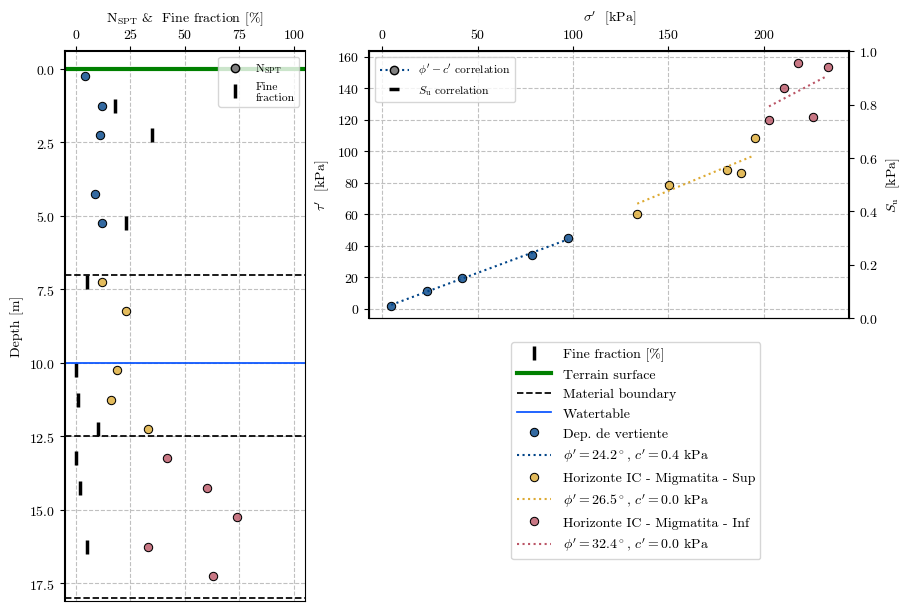
Plotting the processed data

plot_processing(df, mat_depths, wt_depth)