© 2024 Exneyder A. Montoya-Araque, Daniel F. Ruiz y Universidad EAFIT.
This notebook can be interactively run in Google - Colab.
This notebook evaluates susceptibility through the information value method and the proposed methodology by Ciurleo et al. (2016) consisting of two steps. First, the production of a landslide susceptibility computational map, and second, the output of a susceptibility map for zoning purposes; in the latter, the terrain computational units (TCU) of the first map are aggregated into a larger terrain zoning unit (TZU).
The material used here has pedagogical-only purposes and was taken from the tutorial resources provided at the 2023 LAndslide Risk Assessment and Mitigation -LARAM- school.
Required modules and global setup for plots
import os
import sys
import shutil
import subprocess
from IPython import get_ipython

if 'google.colab' in str(get_ipython()):
    print('Running on CoLab. Installing the required modules...')
    from subprocess import run
    # run('pip install ipympl', shell=True);
    run('pip install rasterio', shell=True);
    from google.colab import output, files
    output.enable_custom_widget_manager()
else:
    import tkinter as tk
    from tkinter.filedialog import askopenfilename

import numpy as np
import pandas as pd
import scipy as sp
import matplotlib.pyplot as plt
import matplotlib as mpl
from sklearn.metrics import roc_curve, roc_auc_score
import rasterio

# Figures setup
# %matplotlib widget
mpl.rcParams.update({
    "font.family": "serif",
    "font.serif": ["Computer Modern Roman", "cmr", "cmr10", "DejaVu Serif"],  # or
    "mathtext.fontset": "cm",  # Use Computer Modern fonts for math
    "axes.formatter.use_mathtext": True,  # Use mathtext for axis labels
    "axes.unicode_minus": False,   # Use standard minus sign instead of a unicode character
})
tol_cols = ["#004488", "#DDAA33", "#BB5566"]

n_classes = 8  # number of classes to divide the conditioning factors
Functions
def load_tiff(path):
    with rasterio.open(path) as src:
        raster = src.read(1).astype(float)
        raster[raster == src.nodata] = np.nan
        return raster, src.transform, src.crs, src.bounds

def plot_field(field, bounds, title=None, cmap='viridis'):
    fig, ax = plt.subplots()
    if len(np.unique(field)) > n_classes:  # Plot contours only if it's a continuous conditioning factor
        im = ax.imshow(field, cmap=cmap, extent=(bounds.left, bounds.right, bounds.bottom, bounds.top))
        # ax.contour(field, colors='black', alpha=0.5, origin='image',
        #         extent=(bounds.left, bounds.right, bounds.bottom, bounds.top))
        cbar = plt.colorbar(mappable=im, ax=ax, label=title)
    if len(np.unique(field)) <= n_classes:
        field_r, ticks_r, cmap_r = extract_from_discrete(field, cmap)
        im = ax.imshow(field_r, cmap=cmap_r, extent=(bounds.left, bounds.right, bounds.bottom, bounds.top))
        cbar = plt.colorbar(mappable=im, ax=ax, label=title, ticks=ticks_r)
    fig.canvas.header_visible = False
    fig.canvas.toolbar_position = 'bottom'
    plt.show()
    return fig

def extract_from_discrete(field, cmap='viridis'):
    ticks = np.unique(field)[~np.isnan(np.unique(field))]  # For colorbar
    n = len(ticks)
    field_r = np.full_like(field, np.nan)  # Empty reclasified field
    ticks_r = np.arange(n)  # Ticks to use in reclasified field
    for i in ticks_r:  #  Fill reclasified field
        field_r[field == ticks[i]] = i
    cmap_r = plt.colormaps.get_cmap(cmap).resampled(n)  # type: ignore
    return field_r, ticks_r, cmap_r

def nan_gaussian_filter(data, sigma):
    nan_mask = np.isnan(data)

    # Replace NaNs with 0 for convolution
    data_filled = np.where(nan_mask, 0, data)

    # Create a weight mask of valid data
    weights = (~nan_mask).astype(float)

    # Apply Gaussian filter to data and weights
    data_filtered = sp.ndimage.gaussian_filter(data_filled, sigma=sigma, mode='constant', cval=0.0)
    weights_filtered = sp.ndimage.gaussian_filter(weights, sigma=sigma, mode='constant', cval=0.0)

    # Normalize the result
    with np.errstate(invalid='ignore', divide='ignore'):
        normalized = data_filtered / weights_filtered
        normalized[weights_filtered == 0] = np.nan  # Restore NaNs
    normalized = np.where(nan_mask, np.nan, normalized)  # Restore NaNs in the original positions
    return normalized
Reading the input data
If working on Google Colab, set the testing_data variable in the following cell as False. Then you will be asked to upload your own raster files.
testing_data = True  # Set to False to use the GUI to load the data from an external file

local_data = False  # Set to True to load the data from a local directory either in Colab or in a local machine.

if local_data:
    local_folder_conditioning_factors = "local_folder_conditioning_factors/"
    local_folder_inventory = "local_folder_inventory/"
    os.makedirs(local_folder_conditioning_factors, exist_ok=True)
    os.makedirs(local_folder_inventory, exist_ok=True)
else:
    local_folder_conditioning_factors = "./"
    local_folder_inventory = "./"
Loading testing data
if testing_data:
url = "https://github.com/eamontoyaa/data4testing/raw/refs/heads/main/susceptibility/"
# Load the data (conditioning factors)
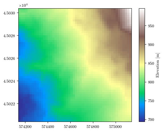
elevation, transform, crs, bounds = load_tiff(f"{url}/elevation.tif")
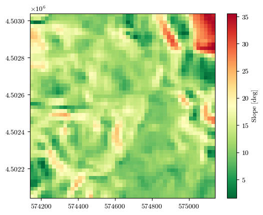
slope, _, _, _ = load_tiff(f"{url}/slope.tif")
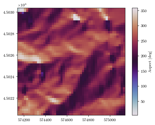
aspect, _, _, _ = load_tiff(f"{url}/aspect.tif")
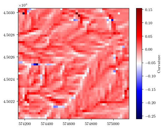
curvature, _, _, _ = load_tiff(f"{url}/curvature.tif")
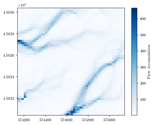
flow_acc, _, _, _ = load_tiff(f"{url}/flow_acc.tif")
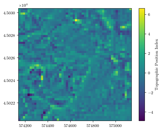
tpi, _, _, _ = load_tiff(f"{url}/tpi.tif")
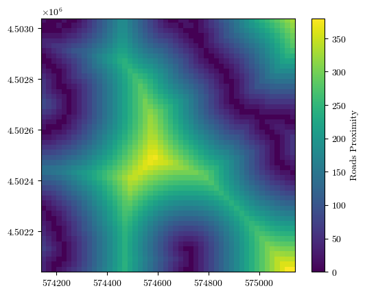
roads_prox, _, _, _ = load_tiff(f"{url}/roads_prox.tif")
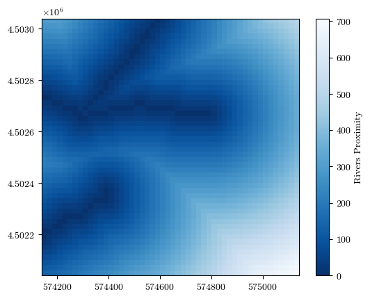
rivers_prox, _, _, _ = load_tiff(f"{url}/rivers_prox.tif")
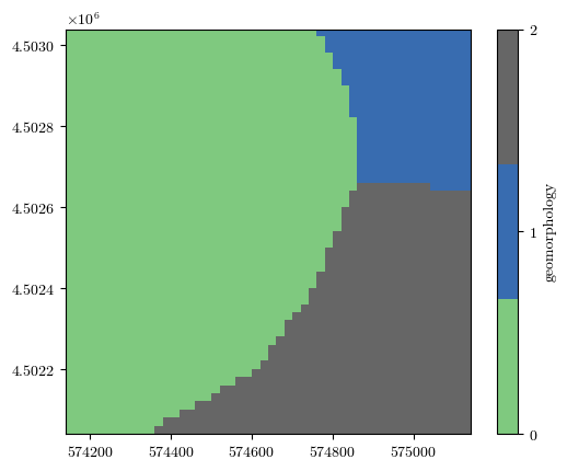
geomorphology, _, _, _ = load_tiff(f"{url}/geomorphology.tif")
df_cond_fact = pd.DataFrame({
'elevation': elevation.flatten(),
'slope': slope.flatten(),
'aspect': aspect.flatten(),
'curvature': curvature.flatten(),
'flow_acc': flow_acc.flatten(),
'tpi': tpi.flatten(),
'roads_prox': roads_prox.flatten(),
'rivers_prox': rivers_prox.flatten(),
'geomorphology': geomorphology.flatten(),
})
independent_vars = df_cond_fact.columns.to_list()
independent_vars_types = ['c', 'c', 'c', 'c', 'c', 'c', 'c', 'c', 'd']
# Mask of NaN values for all the conditioning factors
mask_nan = df_cond_fact.isna().any(axis=1)
mask_nan_mtx = mask_nan.values.reshape(elevation.shape)
# Landslides
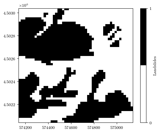
landslides, _, _, _ = load_tiff(f"{url}/landslides.tif")
landslides[np.isnan(landslides)] = 0
landslides[mask_nan_mtx] = np.nan
df_landslides = pd.Series(landslides.flatten())
# Plot the data
fig = plot_field(elevation, bounds, title='Elevation [m]', cmap='terrain')
fig = plot_field(slope, bounds, title='Slope [deg]', cmap='RdYlGn_r')
fig = plot_field(aspect, bounds, title='Aspect [deg]', cmap='twilight')
fig = plot_field(curvature, bounds, title='Curvature', cmap='seismic')
fig = plot_field(flow_acc, bounds, title='Flow Accumulation', cmap='Blues')
fig = plot_field(tpi, bounds, title='Topographic Position Index', cmap='viridis')
fig = plot_field(roads_prox, bounds, title='Roads Proximity', cmap='viridis')
fig = plot_field(rivers_prox, bounds, title='Rivers Proximity', cmap='Blues_r')
fig = plot_field(geomorphology, bounds, title='geomorphology', cmap='Accent')
fig = plot_field(landslides, bounds, title='Landslides', cmap='binary')
Uploading the raster files of conditioning factors
if testing_data is False:
    outputs_folder = "outputs"
    os.makedirs(outputs_folder, exist_ok=True)
    df_cond_fact = pd.DataFrame()
    # List the files to load
    if testing_data is False and local_data is False:
        cond_factors_files = files.upload()
        local_folder_conditioning_factors = os.getcwd()
    elif local_data:
        cond_factors_files = os.listdir(local_folder_conditioning_factors)

    # Load the conditioning factors and plot them
    for file in cond_factors_files:
        if file.endswith('.tif'):
            file_name = file.split('.')[0].split(' ')[0]
            raster, transform, crs, bounds = load_tiff(os.path.join(local_folder_conditioning_factors, file))
            print(f"Loaded {file_name} with shape {raster.shape}")
            fig = plot_field(raster, bounds, title=file_name)
            df_cond_fact[file_name] = raster.flatten()

    # Determine the type of each conditioning factor (continuous or discrete)
    independent_vars = df_cond_fact.columns.to_list()
    independent_vars_types = ['c']*len(independent_vars)
    # If unique values are less than or equal to n_classes, then it is a discrete variable
    for idx, col in enumerate(independent_vars):
        if len(df_cond_fact[col].unique()) <= n_classes:
            independent_vars_types[idx] = 'd'

    # Mask of NaN values for all the conditioning factors
    mask_nan = df_cond_fact.isna().any(axis=1)
    mask_nan_mtx = mask_nan.values.reshape(raster.shape)
Uploading the raster files of landslides
if testing_data is False:
    df_landslides = pd.Series()
    # List the file to load (It'll read the first file uploaded/stored, so make sure to upload only the landslides inventory)
    if testing_data is False and local_data is False:
        landslides_files = files.upload()
        landslides, transform, crs, bounds = load_tiff(list(landslides_files.keys())[0])
    elif local_data:
        landslides_files = os.listdir(local_folder_inventory)
        landslides, transform, crs, bounds = load_tiff(os.path.join(local_folder_inventory, landslides_files[0]))
    # Process the landslides inventory
    landslides[landslides != 1] = 0
    df_landslides = pd.Series(landslides.flatten())
    # Plot the landslides inventory
    fig = plot_field(landslides, bounds, title='Landslides', cmap='binary')
mask_nan_cond_fact = df_cond_fact.isna().any(axis=1)
mask_nan_landslides = df_landslides.isna()
mask_nan = mask_nan_cond_fact | mask_nan_landslides
# Replace the NaN values in the conditioning factors and landslides with NaN
df_cond_fact.loc[mask_nan] = np.nan
df_landslides.loc[mask_nan] = np.nandf_cond_factindependent_vars_types['c', 'c', 'c', 'c', 'c', 'c', 'c', 'c', 'd']df_landslides0 0.0
1 0.0
2 0.0
3 0.0
4 0.0
...
2495 0.0
2496 0.0
2497 0.0
2498 0.0
2499 0.0
Length: 2500, dtype: float64Percentile class for each independent variable
The independent variables are classified according to a quantile criterion employing 8 classes
percentages = np.linspace(0, 100, n_classes+1)  # percentages for the percentiles to compute
df_cond_fact_p = df_cond_fact.copy()

for n_iv, iv in enumerate(independent_vars): # Variable whose percentiles is being classified
    p_class = np.full_like(df_landslides.to_numpy(), fill_value=-1, dtype=int)  # percentile classes
    if independent_vars_types[n_iv] == 'c':
        percentiles = np.nanpercentile(df_cond_fact[iv], percentages, method='linear')  # percentiles that limit the clases
        for p in np.arange(n_classes):
            p_class[df_cond_fact[iv].to_numpy() >= percentiles[p]] = p
    elif independent_vars_types[n_iv] == 'd':
        uvals = np.unique(df_cond_fact[iv])
        for n_uval, uval in enumerate(uvals):
            p_class[df_cond_fact[iv] == uval] = n_uval
    if any(p_class == -1):
        n_unclass = np.sum(p_class==-1)
        print(f"There are {n_unclass} TCUs in the '{iv}' independent variable without percentile classification")
    df_cond_fact_p[iv] = p_class  # This plus one is to math the tutorial nomenclature

df_cond_fact_p
There are 2 TCUs in the 'elevation' independent variable without percentile classification
There are 2 TCUs in the 'slope' independent variable without percentile classification
There are 2 TCUs in the 'aspect' independent variable without percentile classification
There are 2 TCUs in the 'curvature' independent variable without percentile classification
There are 2 TCUs in the 'flow_acc' independent variable without percentile classification
There are 2 TCUs in the 'tpi' independent variable without percentile classification
There are 2 TCUs in the 'roads_prox' independent variable without percentile classification
There are 2 TCUs in the 'rivers_prox' independent variable without percentile classification
There are 2 TCUs in the 'geomorphology' independent variable without percentile classification
→ TCUs belonging to the class of the independent variable 
→ Number of TCUs with landslides belonging to the class of the independent variable
→ Number of TCUs without landslides belonging to the class of the independent variable
# number of TCUs with landslides belonging to the class j of the independent variable Vi
Fij = np.zeros((n_classes, len(independent_vars)))
# number of TCUs without landslides belonging to the class j of the independent variable Vi
NFij = np.zeros((n_classes, len(independent_vars)))

for i in np.arange(n_classes):  # iterate over percentile classes (rows)
    for j, iv in enumerate(independent_vars): # iterate over IV classes (columns)
        Fij[i, j] = np.nansum(np.logical_and(df_cond_fact_p[iv]==i, df_landslides==1))
        NFij[i, j] = np.nansum(np.logical_and(df_cond_fact_p[iv]==i, df_landslides==0))

# number of TCUs belonging to the class j of the independent variable Vi
Nij = Fij + NFij

pd.DataFrame(Nij, columns=independent_vars, index=[f'Class {i}' for i in np.arange(n_classes)])→ Weight of the class of the independent variable 
→ Density of landslides within class of the independent variable
→ Average density of landslides within the test area
Dij = Fij / Nij
Ftot = np.nansum(Fij, axis=0)
NFtot = np.nansum(NFij, axis=0)
Ntot = Ftot + NFtot
Dast = Ftot / Ntot
Wij = np.log10(Dij / Dast)
# Correct weight where no landslides occurred
Wij_inf = np.isinf(Wij)
Wij[Wij_inf] = np.floor(np.nanmin(Wij[~Wij_inf]))

pd.DataFrame(Wij, columns=independent_vars, index=[f'Class {i}' for i in np.arange(n_classes)])
/tmp/ipykernel_52833/3450856213.py:1: RuntimeWarning: invalid value encountered in divide
Dij = Fij / Nij
→ Susceptibility index
df_cond_fact_w = df_cond_fact_p.copy()
for j, iv in enumerate(independent_vars): # iterate over independent variables (columns)
    df_cond_fact_w[iv] = Wij[df_cond_fact_p[iv], j]
df_cond_fact_w.loc[mask_nan] = np.nan
df_cond_fact_w["ISTCU"] = df_cond_fact_w.sum(axis=1)
df_cond_fact_w.loc[mask_nan, "ISTCU"] = np.nan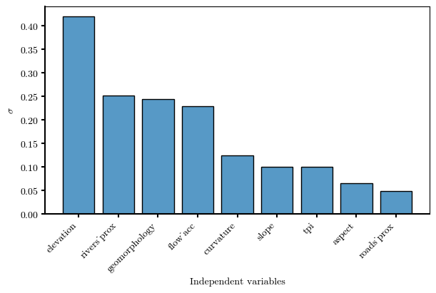
df_cond_fact_w→ statistical indicator to assess the discriminant capability of 
n = np.sum(~np.isnan(Wij), axis=0)  # Number of classes of the independent variable Vi
Wij_ast = Wij * Nij / (Ntot / n)  # normalized value of the weight assigned to the class j of the independent variable Vi
Wi = np.nanmean(Wij, axis=0)  # average value of the weights assigned to the classes of the independent variable Vi
sigma = np.sqrt(np.nansum((Wij_ast - Wi)**2, axis=0) / (n - 1))

# sigma to Series with variable names
sigma_series = pd.Series(sigma, index=independent_vars)
# Order sigma descending
sigma_sorted = sigma_series.sort_values(ascending=False)
sigma_sorted
elevation 0.419273
rivers_prox 0.251950
geomorphology 0.243137
flow_acc 0.228635
curvature 0.123769
slope 0.100160
tpi 0.099654
aspect 0.064685
roads_prox 0.048868
dtype: float64# Bar plot representing sigma
fig, ax = plt.subplots(figsize=(6, 4), layout='constrained')
ax.bar(sigma_sorted.index, sigma_sorted.values,
color=mpl.colors.to_rgba('C0', alpha=0.75), edgecolor='black')
ax.set(ylabel='$\\sigma$', xlabel='Independent variables')
# rotate x labels
ax.set_xticklabels(sigma_sorted.index, rotation=45, ha='right')
ax.spines[["bottom", "left"]].set_linewidth(1.5)
ax.tick_params(width=1.5)
fig.canvas.header_visible = False
fig.canvas.toolbar_position = 'bottom'
plt.show()/tmp/ipykernel_52833/730343487.py:7: UserWarning: set_ticklabels() should only be used with a fixed number of ticks, i.e. after set_ticks() or using a FixedLocator.
ax.set_xticklabels(sigma_sorted.index, rotation=45, ha='right')
Visualize the spatial distribution of the susceptibility index
# Define your colors
colors = ['xkcd:dull green', 'xkcd:dull yellow', 'xkcd:dull pink']
# Create a colormap
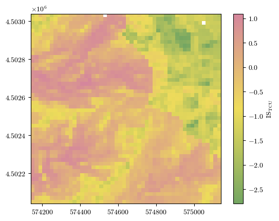
cmap = mpl.colors.LinearSegmentedColormap.from_list("custom_dull_cmap", colors)Raw results for terrain computational units (TCU)
ISTCU = np.reshape(df_cond_fact_w['ISTCU'].to_numpy(), landslides.shape)

fig = plot_field(ISTCU, bounds, title='IS$_\\mathrm{TCU}$', cmap=cmap)#'Spectral_r')
Processed results for larger terrain zoning unit (TZU)
The focal statistics used here is a 2D Gaussian filter with standard deviation used to control the degree of smoothness.
To visualize the landslide boundaries over the map, uncomment the code in the following cell.
ISTZU = nan_gaussian_filter(ISTCU, sigma=1)

mask_nan_border = np.isnan(ISTZU).flatten()
df_cond_fact_w["ISTZU"] = ISTZU.flatten()

fig = plot_field(ISTZU, bounds, title='IS$_\\mathrm{TZU}$', cmap=cmap)#'Spectral_r')

# ax = fig.gca()
# ax.contour(landslides, colors='black', alpha=0.5, origin='image', levels=0, linewidths=5,
#            extent=(bounds.left, bounds.right, bounds.bottom, bounds.top))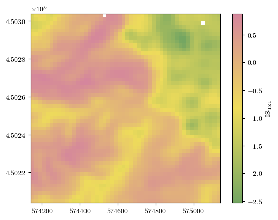
Export results to raster file
To save the susceptibility index map to a raster file, set the want2save variable in the next cell as True.
if testing_data is False:
    src = os.path.join(local_folder_inventory, list(landslides_files.keys())[0])
    dst = os.path.join(outputs_folder, "ISTZU.tif")
    shutil.copy(src, dst)
    # Open the new raster in write mode
    with rasterio.open(dst, 'r+') as dst:
        dst.write(ISTZU, 1)  # Replace the existing array with the modified array
Performance validation of the susceptibility model
fig, ax = plt.subplots(ncols=1, nrows=1, figsize=(5, 5), layout='constrained')
plt.plot([0, 1], [0, 1], 'k--')

fpr, tpr, thresholds = roc_curve(df_landslides.loc[~mask_nan], df_cond_fact_w.loc[~mask_nan, "ISTZU"])  # Calculate the ROC curve
auc_score = roc_auc_score(df_landslides.loc[~mask_nan], df_cond_fact_w.loc[~mask_nan, "ISTZU"])  # Calculate the AUC score
ax.plot(fpr, tpr, label=f'AUC (ISTZU) = {auc_score:.3f}', c='k')

fpr, tpr, thresholds = roc_curve(df_landslides[~mask_nan], df_cond_fact_w.loc[~mask_nan, "ISTCU"])  # Calculate the ROC curve
auc_score = roc_auc_score(df_landslides[~mask_nan], df_cond_fact_w.loc[~mask_nan, "ISTCU"])  # Calculate the AUC score
ax.plot(fpr, tpr, label=f'AUC (ISTCU) = {auc_score:.3f}')

# All the independent variables
for iv in independent_vars:
    fpr, tpr, thresholds = roc_curve(df_landslides[~mask_nan], df_cond_fact_w.loc[~mask_nan, iv])  # Calculate the ROC curve
    auc_score = roc_auc_score(df_landslides[~mask_nan], df_cond_fact_w.loc[~mask_nan, iv])  # Calculate the AUC score
    ax.plot(fpr, tpr, label=f'AUC ({iv}) = {auc_score:.3f}')

ax.set_xlabel('False Positive Rate')
ax.set_ylabel('True Positive Rate')
ax.set_aspect('equal')
ax.legend()
ax.grid(True, color='0.3', ls='--', lw=0.7)

fig.canvas.header_visible = False
fig.canvas.toolbar_position = 'bottom'
plt.show()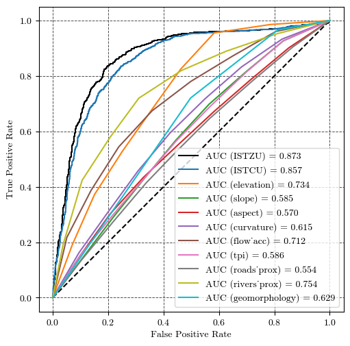
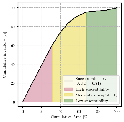
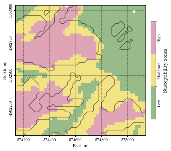
Landslide susceptibility zonation
colors = ['xkcd:dull green', 'xkcd:dull yellow', 'xkcd:dull pink',]# 'xkcd:dull red', ]
cmap_zones = mpl.colors.ListedColormap(colors)
bounds_zonation = [-0.5, 0.5, 1.5, 2.5]  # Boundaries between values
norm = mpl.colors.BoundaryNorm(bounds_zonation, cmap_zones.N)
# cmap_zones
low_to_mod_perc = 95 # [%] Percentage of landslide cells at high and moderate susceptibility → (1 - low_to_mod_perc) is the percentage of landslide cells at low susceptibility
mod_to_high_perc = 60 # [%] Percentage of landslide cells at high susceptibilityinventory, zonation_index = df_landslides.loc[~mask_nan].to_numpy(), df_cond_fact_w.loc[~mask_nan, "ISTZU"].to_numpy()
# Sort probability values in descending order
sorted_indices = np.argsort(-zonation_index) # Descending order
sorted_index = zonation_index[sorted_indices]
sorted_inventory = inventory[sorted_indices]
# Compute cumulative percentage of inventory covered
total_inventory = np.sum(inventory)
cumulative_inventory = np.cumsum(sorted_inventory) / total_inventory
# Compute cumulative percentage of the area
cumulative_area = np.linspace(0, 1, len(sorted_index))
# Determine susceptibility zones based on probability thresholds
idx_LM = np.searchsorted(cumulative_inventory, low_to_mod_perc / 100) # index where 50% of inventory are included
idx_MH = np.searchsorted(cumulative_inventory, mod_to_high_perc / 100) # index where 90% of inventory are included
threshold_LM = sorted_index[idx_LM]
threshold_MH = sorted_index[idx_MH]
susceptibility_thresholds = [threshold_LM, threshold_MH]
# Performance metrics
y_test_index = zonation_index
y_true = inventory
# ROC curve for the probability of failure
fpr, tpr, thresholds = roc_curve(y_true, y_test_index)
auc_score_index = roc_auc_score(y_true, y_test_index)
auc_score_index = np.trapezoid(cumulative_inventory, cumulative_area)
print(f"ROC AUC Score: {auc_score_index:.4f}")
# Plot Success Rate Curve (SRC)
fig, ax = plt.subplots(ncols=1, nrows=1, layout='constrained', figsize=(5, 4))# 1:1 line
# ax.plot([0, 100], [0, 100], '--k', lw=1.5)
ax.plot(cumulative_area*100, cumulative_inventory*100, c='k', lw=1.5,
label="Success rate curve\n(AUC = {:.2f})".format(auc_score_index))
# label="Curva de exito\n(AUC = {:.2f})".format(auc_score_index))
# Fill the area under the curve for the thresholds
# High susceptibility threshold
ax.fill_between(cumulative_area[:idx_MH]*100, cumulative_inventory[:idx_MH]*100,
color=colors[-1], alpha=0.6, label="High susceptibility")
# Medium susceptibility threshold
ax.fill_between(cumulative_area[idx_MH:idx_LM]*100, cumulative_inventory[idx_MH:idx_LM]*100,
color=colors[-2], alpha=0.6, label="Moderate susceptibility")
# Low susceptibility threshold
ax.fill_between(cumulative_area[idx_LM:]*100, cumulative_inventory[idx_LM:]*100,
color=colors[0], alpha=0.6, label="Low susceptibility")
ax.set_xlabel("Cumulative Area [%]")
ax.set_ylabel("Cumulative inventory [%]")
ax.legend(loc='lower right')
ax.grid(True, ls='--')
ax.spines[["bottom", "left"]].set_linewidth(1.5)
ax.tick_params(width=1.5)
ax.set_aspect('equal')
# fig.canvas.header_visible = False
# fig.canvas.toolbar_position = 'bottom'
plt.show()
ROC AUC Score: 0.7061
susceptibility_zonation = np.digitize(ISTZU, bins=susceptibility_thresholds, right=True).astype(float)
susceptibility_zonation[mask_nan_mtx] = np.nan

fig, ax = plt.subplots(1, 1, layout="constrained")

# Plot rasters
# ax.imshow(HSD, cmap='Grays_r', alpha=1, extent=extent)
extent=(bounds.left, bounds.right, bounds.bottom, bounds.top)
im = ax.imshow(susceptibility_zonation, cmap=cmap_zones, norm=norm, alpha=0.75, extent=extent)
landslide_contour = ax.contour(landslides, colors='black', alpha=0.5, origin='image', levels=[0.5], lw=1.5, extent=extent)
# Add colorbar
cbar = plt.colorbar(im, ax=ax, orientation='vertical', shrink=0.75, pad=0.03, ticks=[0, 1, 2])
_ = cbar.ax.set_yticklabels(['Low', 'Moderate', 'High'])
cbar.set_label('Susceptibility zones', rotation=90, size="large")
cbar.ax.tick_params(axis="y", labelrotation=90, pad=1.5)
[label.set_va("center") for label in cbar.ax.get_yticklabels()]

# Figure aesthetics
ax.grid(True, ls=':', lw=0.5, color='k')
ax.spines[["bottom", "left"]].set_linewidth(1.5)
ax.set_xlabel('East [m]')
ax.xaxis.set_major_formatter(mpl.ticker.ScalarFormatter(useMathText=False))
ax.xaxis.set_major_locator(mpl.ticker.MaxNLocator(nbins=5))
ax.ticklabel_format(style='plain', axis='x')
ax.set_ylabel('North [m]')
ax.yaxis.set_major_formatter(mpl.ticker.ScalarFormatter(useMathText=False))
ax.ticklabel_format(style='plain', axis='y')  # or axis='x'
plt.setp(ax.get_yticklabels(), rotation=90, ha='right', va='center')
ax.yaxis.set_major_locator(mpl.ticker.MaxNLocator(nbins=4))
ax.tick_params(width=1.5)

plt.show()
/tmp/ipykernel_52833/4174874169.py:10: UserWarning: The following kwargs were not used by contour: 'lw'
  landslide_contour = ax.contour(landslides, colors='black', alpha=0.5, origin='image', levels=[0.5], lw=1.5, extent=extent)
if testing_data is False:
    src = os.path.join(local_folder_inventory, list(landslides_files.keys())[0])
    dst = os.path.join(outputs_folder, "susceptibility_zonation.tif")
    shutil.copy(src, dst)
    # Open the new raster in write mode
    with rasterio.open(dst, 'r+') as dst:
dst.write(susceptibility_zonation, 1) # Replace the existing array with the modified array- Ciurleo, M., Calvello, M., & Cascini, L. (2016). Susceptibility Zoning of Shallow Landslides in Fine Grained Soils by Statistical Methods. Catena, 139, 250–264. 10.1016/j.catena.2015.12.017