Mohr circle and stress paths - Slope stability notes

This notebook can be interactively run in Google - Colab.

Required modules and global setup for plots¶

import ast
import numpy as np
import matplotlib.pyplot as plt
import matplotlib as mpl
from ipywidgets import widgets as wgt
from IPython import get_ipython
from IPython.display import display

if 'google.colab' in str(get_ipython()):
    print('Running on CoLab. Installing the required modules...')
    from subprocess import run
    # run('pip install ipympl', shell=True);
    from google.colab import output
    output.enable_custom_widget_manager()
    
# Figures setup
# %matplotlib widget
mpl.rcParams.update({
    "font.family": "serif",
    "font.serif": ["Computer Modern Roman", "cmr", "cmr10", "DejaVu Serif"],  # or 
    "mathtext.fontset": "cm",  # Use Computer Modern fonts for math
    "axes.formatter.use_mathtext": True,  # Use mathtext for axis labels
    "axes.unicode_minus": False,   # Use standard minus sign instead of a unicode character
})

Funciones¶

def get_xy_from_angle(angle, r, c):
    x, y = r * np.cos(2*np.deg2rad(angle)) + c, r * np.sin(2*np.deg2rad(angle))
    return x, y

def plot_mohr_circle(
    𝜎_xx, 𝜎_yy, 𝜏_xy, plot_envelope=False, envelope={'c': 5, '𝜙': 27},
    plot_pole=False, plot_plane=False, 𝛼=0, xlim=None, ylim=None, **kwargs
):
    if type(envelope) == str:  # This is for interpreting it from the widget
        envelope = ast.literal_eval('{' + envelope + '}')

    c = 0.5 * (𝜎_xx + 𝜎_yy)
    r = np.sqrt((𝜎_xx - c) ** 2 + 𝜏_xy**2)
    𝜎_1 = r * np.cos(0) + c
    𝜎_3 = r * np.cos(np.pi) + c

    tension_state = {
        "𝜎_1": 𝜎_1,
        "𝜎_3": 𝜎_3,
        "𝜎_xx": 𝜎_xx,
        "𝜎_yy": 𝜎_yy,
        "𝜏_xy": 𝜏_xy,
        "s": 0.5 * (𝜎_1 + 𝜎_3),
        "t": 0.5 * (𝜎_1 - 𝜎_3),
        "p": 1 / 3 * (𝜎_1 + 2 * 𝜎_3),
        "q": 𝜎_1 - 𝜎_3,
    }

    angles4circ = np.linspace(0, 2 * np.pi, 200)

    fig, ax = plt.subplots(ncols=1, nrows=1, figsize=kwargs.get('figsize'))
    ax.plot(r * np.cos(angles4circ) + c, r * np.sin(angles4circ), c="k")  # Mohr circle
    ax.axhline(y=0, c="k")

    params = {'ls': "", "fillstyle": 'none', "markeredgewidth": 2, "ms": 7}
    # Cartesian stresses 𝜎_xx, 𝜏_xy and 𝜎_yy, (-)𝜏_xy
    label = ("$\\sigma_{xx}=$" + f"{𝜎_xx:.1f}" + ",\n$\\tau_{xy}=$" + f"{𝜏_xy:.1f}")
    ax.plot(𝜎_xx, 𝜏_xy, c="C1", marker="s", label=label, **params)
    label = ("$\\sigma_{yy}=$" + f"{𝜎_yy:.1f}" + ",\n$\\tau_{yx}=$" + f"{𝜏_xy:.1f}")
    ax.plot(𝜎_yy, -𝜏_xy, c="C0", marker="s", label=label, **params)
    # Principal stresses 𝜎_1, 𝜎_3
    label = "$\\sigma_{1}=$" + f"{𝜎_1:.1f}"  # 𝜎_1
    ax.plot(𝜎_1, 0, c="C3", marker= "o", label=label, **params)
    label = "$\\sigma_{3}=$" + f"{𝜎_3:.1f}"  # 𝜎_3
    ax.plot(𝜎_3, 0, c="C4", marker= "o", label=label, **params)
    ax.plot(c, 0, ls="", c="k", marker=(8, 2, 0), ms=10,  # Mean stress
        label="$\\sigma_\\mathrm{m}=$" + f"{c:.1f}")
    label = "$\\tau_\mathrm{max}=$" + f"{r:.1f}"  # 𝜏_max
    ax.plot(c, r, c="C5", marker="v", label=label, **params)

    pole = (𝜎_xx, -1 * 𝜏_xy)
    if plot_pole:  # Pole and stress on a plane
        ax.axvline(x=pole[0], c="C1", ls="-", lw=1.25)
        ax.axhline(y=pole[1], c="C0", ls="-", lw=1.25)
        ax.plot(*pole, ls="", c="k", marker=".", fillstyle='full', ms=7,
            label=f"Pole$_\\sigma={pole[0]:.1f}$,\nPole$_\\tau= {pole[1]:.1f}$")
    if plot_plane:
        𝛽 = 0.5 * np.degrees(np.arctan2(2 * 𝜏_xy, 𝜎_xx - 𝜎_yy))
        𝜃 = 𝛼 + 𝛽
        pl_𝜎, pl_𝜏 = get_xy_from_angle(𝜃, r, c)
        label = f"Plane at {𝛼:.1f}" + "$^{\circ}\\circlearrowleft$\nfrom Plane $\\sigma_x$"
        ax.plot((pl_𝜎, pole[0]), (pl_𝜏, pole[1]), c="C1", ls="--", lw=1.25, label=label)
        label="Plane at $2\\theta=$" + f"{2*𝜃:.1f}" + \
            "$^{\\circ}\\circlearrowleft$\nfrom Plane $\\sigma_1$"
        ax.plot((pl_𝜎, c), (pl_𝜏, 0), c="C3", ls="--", lw=1.25, label=label)
        label = "Stress state on the plane\n" + "$\\sigma_\\mathrm{n}=$" + \
            f"{pl_𝜎:.1f}" + ", $\\tau_\mathrm{n}=$" + f"{pl_𝜏:.1f}"
        ax.plot(pl_𝜎, pl_𝜏, ls="", c="k", marker="o", fillstyle='none', label=label)

    if plot_envelope:  # Failure envelope
        tan_𝜙 = np.tan(np.radians(envelope['𝜙']))
        c_env = envelope['c']
        label = "Failure criterion\n$\\tau_\\mathrm{n}=" + f"{envelope['c']}+" + \
            "\\tan" + f"{envelope['𝜙']}^\\circ" + "\\sigma_\\mathrm{n}$"
        xlim = ax.get_xlim() if xlim is None else xlim
        ylim = ax.get_ylim() if ylim is None else ylim
        x_env = np.array([-9e9, 9e9])
        ax.plot(x_env, tan_𝜙 * x_env + envelope['c'], c="r", label=label)

    ax.legend(loc="center left", bbox_to_anchor=(1, 0.5))
    ax.grid(True, ls="--")
    ax.spines["bottom"].set_linewidth(1.5)
    ax.spines["left"].set_linewidth(1.5)
    ax.set_aspect("equal", anchor=None)
    ax.set(
        xlabel="Normal stress, $\\sigma_\\mathrm{n}$",
        ylabel="Shear stress, $\\tau_\\mathrm{n}$",
        xlim=xlim,
        ylim=ylim
    )
    # display_fig(fig, kwargs.get('static_fig', False))
    return tension_state

def plot_all_mohr_circles(
        stages, envelope={'c': 20, '𝜙': 35}, xlim=None, ylim=None, **kwargs):
    theta = np.linspace(0, 2 * np.pi, 200)
    # sigma = np.linspace(0, 𝜎_1 * factor, 200)
    fig, ax = plt.subplots(ncols=1, nrows=1, figsize=kwargs.get('figsize'))
    for i, st in enumerate(stages):
        𝜎_xx, 𝜎_yy, 𝜏_xy = st['𝜎_xx'], st['𝜎_yy'], st['𝜏_xy']
        c = 0.5 * (𝜎_xx + 𝜎_yy)
        r = np.sqrt((𝜎_xx - c) ** 2 + 𝜏_xy**2)
        𝜎_1 = r * np.cos(0) + c
        𝜎_3 = r * np.cos(np.pi) + c
        # ax.axhline(y=0, xmin=0, xmax=𝜎_1 * factor, c="k")
        ax.plot(r * np.cos(theta) + c, r * np.sin(theta), label=f'Stage {i}')  # Mohr circle
    # Failure envelope
    tan_𝜙 = np.tan(np.radians(envelope['𝜙']))
    c_env = envelope['c']
    label = ("Failure criterion \n $\\tau_\mathrm{n} = "+ f"{c_env} + "
                + "\\tan" + f"{envelope['𝜙']}^\circ" + "\sigma_\mathrm{n}$")
    xlim = ax.get_xlim() if xlim is None else xlim
    ylim = ax.get_ylim() if ylim is None else ylim
    x_env = np.array([-9e9, 9e9])
    ax.plot(x_env, tan_𝜙 * x_env + c_env, c="r", label=label)

    ax.legend(loc="center left", bbox_to_anchor=(1, 0.5))
    ax.grid(True, ls="--")
    ax.spines["bottom"].set_linewidth(1.5)
    ax.spines["left"].set_linewidth(1.5)
    # ax.axis("equal")
    ax.set_aspect("equal", adjustable=None, anchor='C')
    ax.set(
        xlabel="Normal stress, $\sigma_\mathrm{n}$",
        ylabel="Shear stress, $\\tau_\mathrm{n}$",
        xlim=xlim,
        ylim=ylim)
    # display_fig(fig, kwargs.get('static_fig', False))
    return

def plot_stress_path(stages, envelope={"c": 10, "𝜙": 30}, **kwargs):
    # Mohr-Coulomb envelope
    phi_r = np.radians(envelope["𝜙"])
    c = envelope["c"]
    𝜎1, 𝜎3, s, t, p, q = [], [], [], [], [], []
    for st in stages:
        𝜎1.append(st["𝜎_1"])
        𝜎3.append(st["𝜎_3"])
        s.append(st["s"])
        t.append(st["t"])
        p.append(st["p"])
        q.append(st["q"])

    fig, (ax0, ax1, ax2) = plt.subplots(ncols=3, nrows=1, figsize=kwargs.get('figsize'))
    quiver = lambda x, y: (
        0.5 * (x[1:] + x[:-1]),
        0.5 * (y[1:] + y[:-1]),
        np.diff(x)/np.sqrt(np.diff(x)**2+np.diff(y)**2),
        np.diff(y)/np.sqrt(np.diff(x)**2+np.diff(y)**2),
    )

    x_env = np.array([-9e9, 9e9])
    # 𝜎_1, 𝜎_3
    𝜎1, 𝜎3 = np.array(𝜎1), np.array(𝜎3)
    ax0.plot(𝜎3, 𝜎1, ls="--", c="k", marker="o", mfc="tomato", lw=0.75)
    ax0.quiver(*quiver(𝜎3, 𝜎1), pivot="mid", angles="xy")
    label = (
        "Failure criterion: \n$\sigma_1' =  "
        + "\\frac{2c' \cos \phi'}{1 - \sin \phi'} + "
        + "\sigma_3' \\frac{1 + \sin \phi'}{1 - \sin \phi'} $"
    )
    𝜎1_𝜎3_int = 2 * c * np.cos(phi_r) / (1 - np.sin(phi_r))
    𝜎1_𝜎3_slope = (1 + np.sin(phi_r)) / (1 - np.sin(phi_r))
    ax0.axline(xy1=(0, 𝜎1_𝜎3_int), slope=𝜎1_𝜎3_slope, c="#BB5566", label=label)
    ax0.set(xlabel="$\sigma_{3}'$", ylabel="$\sigma_{1}'$")
    ax0.set_xlim(kwargs.get('xlim')) if 'xlim' in kwargs.keys() else ax0.set_xlim((0, 1.2 * max(𝜎3)))
    ax0.set_ylim(kwargs.get('ylim')) if 'ylim' in kwargs.keys() else ax0.set_ylim((0, 1.2 * max(𝜎1)))
    𝜎3_lim, 𝜎1_lim = np.array(ax0.get_xlim()), np.array(ax0.get_ylim())


    # s, t
    s, t = np.array(s), np.array(t)
    ax1.plot(s, t, ls="--", c="k", marker="o", mfc="tomato", lw=0.75)
    ax1.quiver(*quiver(s, t), pivot="mid", angles="xy")
    label = "Failure criterion: \n$t = c' \cos \phi' + s'\,\sin \phi' $"
    s_t_int = c * np.cos(phi_r)
    s_t_slope = np.sin(phi_r)
    ax1.axline(xy1=(0, s_t_int), slope=s_t_slope, c="#004488", label=label)
    ax1.set(xlabel="$s'$", ylabel="$t$")
    ax1.set_xlim(0.5 * (𝜎1_lim + 𝜎3_lim))
    ax1.set_ylim(0.5 * (𝜎1_lim - 𝜎3_lim))
    
    # p, q
    p, q = np.array(p), np.array(q)
    ax2.plot(p, q, ls="--", c="k", marker="o", mfc="tomato", lw=0.75)
    ax2.quiver(*quiver(p, q), pivot="mid", angles="xy")
    label = (
        "Failure criterion: \n$q =  "
        + "\\frac{6\cos \phi'}{3 - \sin \phi'} +"
        + "\\frac{6\sin \phi'}{3 - \sin \phi'} p'$"
    )
    p_q_int = c * 6 * np.cos(phi_r) / (3 - np.sin(phi_r))
    p_q_slope = 6 * np.sin(np.arctan(phi_r)) / (3 - np.sin(np.arctan(phi_r)))
    ax2.axline(xy1=(0, p_q_int), slope=p_q_slope, c="#DDAA33", label=label)
    ax2.set(xlabel="$p'$", ylabel="$q$")
    ax2.set_xlim(1 / 3 * (𝜎1_lim + 2 * 𝜎3_lim))
    ax2.set_ylim(𝜎1_lim - 𝜎3_lim)

    for ax in (ax0, ax1, ax2):
        ax.legend(loc="upper center", bbox_to_anchor=(0.5, -0.2))
        ax.grid(True, ls=":")
        ax.spines["bottom"].set_linewidth(1.5)
        ax.spines["left"].set_linewidth(1.5)
    # display_fig(fig, kwargs.get('static_fig', False))
    return

0.5 * (180-100)

40.0

Basic example of the Mohr’s circle¶

# plot_mohr_circle(𝜎_xx=30, 𝜎_yy=20, 𝜏_xy=10)
plot_mohr_circle(𝜎_xx=30, 𝜎_yy=20, 𝜏_xy=10, plot_pole=True, plot_plane=True, 𝛼=45)

{'𝜎_1': 36.180339887498945,
 '𝜎_3': 13.819660112501051,
 '𝜎_xx': 30,
 '𝜎_yy': 20,
 '𝜏_xy': 10,
 's': 25.0,
 't': 11.180339887498947,
 'p': 21.273220037500348,
 'q': 22.360679774997894}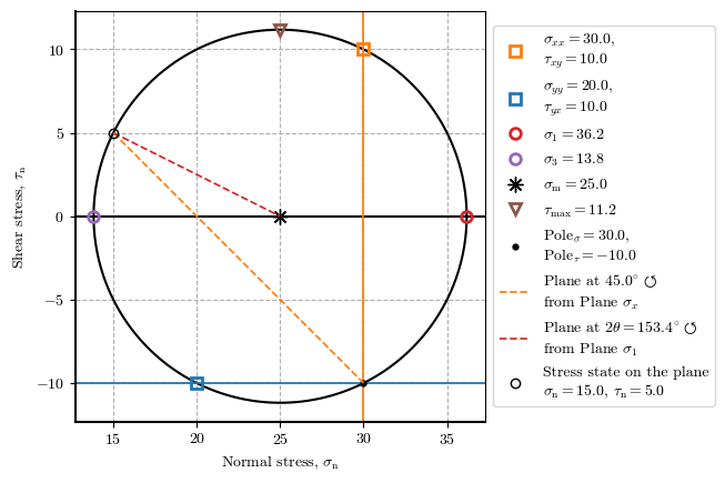

s, l = {'description_width': '60px'}, wgt.Layout(width='400px')
s_env, l_env = {'description_width': '60px'}, wgt.Layout(width='190px')
controls = {
    'σ_xx': wgt.FloatSlider(value=30, min=-10, max=100, description="𝜎_xx", style=s, layout=l),
    'σ_yy': wgt.FloatSlider(value=20, min=-10, max=100, description="𝜎_yy", style=s, layout=l),
    'τ_xy': wgt.FloatSlider(value=10, min=-40, max=40, description="𝜏_xy", style=s, layout=l),
    'plot_pole': wgt.Checkbox(value=False, description="Plot pole?", style=s, layout=l),
    'plot_envelope': wgt.Checkbox(value=False, description="Plot envelope? → ", style=s_env, layout=l_env),
    'envelope': wgt.Text(value="'c': 5, '𝜙': 27", style=s_env, layout=l_env),
    'plot_plane': wgt.Checkbox(value=False, description="Plot a plane? → ", style=s_env, layout=wgt.Layout(width='180px')),
    'α': wgt.FloatSlider(value=45, min=0, max=180, step=0.2, description="α", style={'description_width': '10px'}, layout=wgt.Layout(width='220px')),
    'xlim': wgt.FloatRangeSlider(value=[10, 40], min=-50, max=100, step=.5, description='x-axis:', readout_format='.0f', style=s, layout=l),
    'ylim': wgt.FloatRangeSlider(value=[-15, 15], min=-100, max=100, step=.5, description='y-axis:', readout_format='.0f', style=s, layout=l),
    'static_fig': wgt.Checkbox(value=True, description='Non-vector image (improve widget performance)', disabled=False, style=s, layout=l)
}
c_all = list(controls.values())
c_env = [wgt.HBox(c_all[4:6])]
c_pln = [wgt.HBox(c_all[6:8])]
c = c_all[:4] + c_env + c_pln+ c_all[8:]
fig = wgt.interactive_output(plot_mohr_circle, controls)
wgt.HBox((wgt.VBox(c), fig), layout=wgt.Layout(align_items='center'))

Tool 01¶

Stresses state for the same stage at different points.

ptX_stg3 = plot_mohr_circle(𝜎_xx=15, 𝜎_yy=50, 𝜏_xy=3, envelope={'c': 10, '𝜙': 30}, plot_envelope=True, xlim=(00, 200), ylim=(-60, 60), plot_pole=True, figsize=[7.5, 3.5])
ptY_stg3 = plot_mohr_circle(𝜎_xx=30, 𝜎_yy=85, 𝜏_xy=7.5, envelope={'c': 10, '𝜙': 30}, plot_envelope=True, xlim=(00, 200), ylim=(-60, 60), plot_pole=True, figsize=[7.5, 3.5])
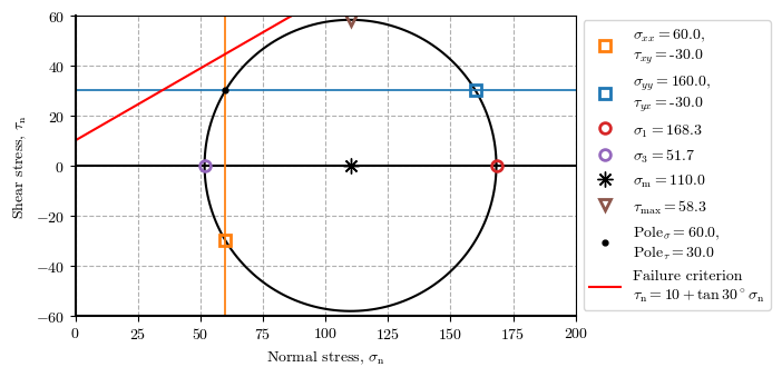
ptZ_stg3 = plot_mohr_circle(𝜎_xx=60, 𝜎_yy=160, 𝜏_xy=-30, envelope={'c': 10, '𝜙': 30}, plot_envelope=True, xlim=(00, 200), ylim=(-60, 60), plot_pole=True, figsize=[7.5, 3.5])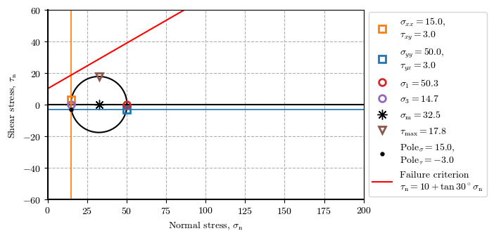

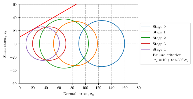
Tool 02¶

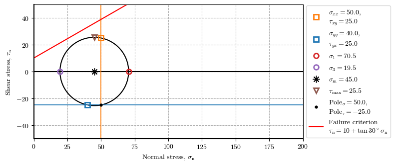
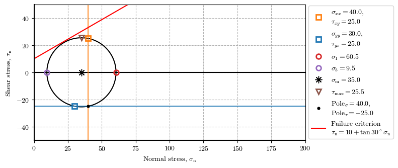
Stresses state for at a point during different stages.

ptX_stg0 = plot_mohr_circle(𝜎_xx=90, 𝜎_yy=160, 𝜏_xy=0, envelope={'c': 10, '𝜙': 30}, plot_envelope=True, xlim=(0, 200), ylim=(-50, 50), plot_pole=True, figsize=[8,3.5])
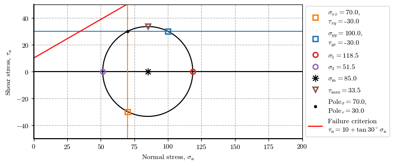
ptX_stg1 = plot_mohr_circle(𝜎_xx=70, 𝜎_yy=100, 𝜏_xy=-30, envelope={'c': 10, '𝜙': 30}, plot_envelope=True, xlim=(0, 200), ylim=(-50, 50), plot_pole=True, figsize=[8,3.5])
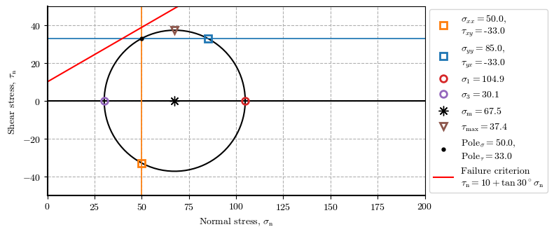
ptX_stg2 = plot_mohr_circle(𝜎_xx=50, 𝜎_yy=85, 𝜏_xy=-33, envelope={'c': 10, '𝜙': 30}, plot_envelope=True, xlim=(0, 200), ylim=(-50, 50), plot_pole=True, figsize=[8,3.5])
ptX_stg3 = plot_mohr_circle(𝜎_xx=50, 𝜎_yy=40, 𝜏_xy=25, envelope={'c': 10, '𝜙': 30}, plot_envelope=True, xlim=(0, 200), ylim=(-50, 50), plot_pole=True, figsize=[8,3.5])
ptX_stg4 = plot_mohr_circle(𝜎_xx=40, 𝜎_yy=30, 𝜏_xy=25, envelope={'c': 10, '𝜙': 30}, plot_envelope=True, xlim=(0, 200), ylim=(-50, 50), plot_pole=True, figsize=[8,3.5])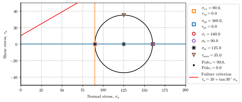

Tool 03¶

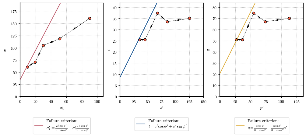
Stress path

ptX_stgs = (ptX_stg0, ptX_stg1, ptX_stg2, ptX_stg3, ptX_stg4)
# All Mohr Circles in one plot
plot_all_mohr_circles(ptX_stgs, envelope={'c': 10, '𝜙': 30}, xlim=(0, 180), ylim=(-60, 60), figsize=[8,3.5])
# Stress paths in trhee spaces
plot_stress_path(ptX_stgs, envelope={'c': 10, '𝜙': 30}, figsize=[12, 4])
# plot_stress_path(ptX_stgs, envelope={'c': 10, '𝜙': 30}, figsize=[12, 4], xlim=(-10, 100), ylim=(-10, 200))