© 2022 Exneyder A. Montoya-Araque, Daniel F. Ruiz and Universidad EAFIT.
This notebook can be interactively run in Google - Colab.
This notebook was developed following the theory presented in Ch. 1 - Book Mohr Circles, Stress Paths and Geotechnics (2nd Ed.) by Parry (2014).
Required modules and global setup for plots
import ast
import numpy as np
import matplotlib.pyplot as plt
import matplotlib as mpl
from ipywidgets import widgets as wgt
from IPython import get_ipython
from IPython.display import display

if 'google.colab' in str(get_ipython()):
    print('Running on CoLab. Installing the required modules...')
    from subprocess import run
    # run('pip install ipympl', shell=True);
    from google.colab import output
    output.enable_custom_widget_manager()

# Figures setup
# %matplotlib widget
mpl.rcParams.update({
    "font.family": "serif",
    "font.serif": ["Computer Modern Roman", "cmr", "cmr10", "DejaVu Serif"],  # or
    "mathtext.fontset": "cm",  # Use Computer Modern fonts for math
    "axes.formatter.use_mathtext": True,  # Use mathtext for axis labels
    "axes.unicode_minus": False,   # Use standard minus sign instead of a unicode character
})
Funciones
def get_strain_state(𝜀_xx, 𝜀_yy, 𝜀_xy):
    c = 0.5 * (𝜀_xx + 𝜀_yy)
    r = np.sqrt((𝜀_xx - c) ** 2 + 𝜀_xy**2)
    𝜀_1 = r * np.cos(0) + c
    𝜀_3 = r * np.cos(np.pi) + c

    strain_state = {
        "𝜀_1": 𝜀_1,
        "𝜀_3": 𝜀_3,
        "𝜀_xx": 𝜀_xx,
        "𝜀_yy": 𝜀_yy,
        "𝜀_xy": 𝜀_xy,
        "𝜀_vol": (𝜀_1 + 𝜀_3),
        "0.5*𝛾_max": r,
        "r": r,
        "c": c
    }
    return strain_state

def get_xy_from_angle(angle, r, c):
    x, y = r * np.cos(2*np.deg2rad(angle)) + c, r * np.sin(2*np.deg2rad(angle))
    return x, y

def plot_mohr_circle(𝜀_xx, 𝜀_yy, 𝜀_xy, plot_pole=False, plot_plane=False, 𝜔=10,
                     xlim=None, ylim=None, **kwargs):
    strain_state = get_strain_state(𝜀_xx, 𝜀_yy, 𝜀_xy)
    pole = (𝜀_xx, -1 * 𝜀_xy)
    angles4circ = np.linspace(0, 2 * np.pi, 200)

    fig, ax = plt.subplots(ncols=1, nrows=1, figsize=kwargs.get('figsize'))
    ax.plot(strain_state['r'] * np.cos(angles4circ) + strain_state['c'],
            strain_state['r'] * np.sin(angles4circ), c="k")  # Mohr circle
    ax.axhline(y=0, c="k")

    params = {'ls': "", "fillstyle": 'none', "markeredgewidth": 2, "ms": 7}
    label = ("$\\varepsilon_{xx}=$" + f"{𝜀_xx:.2f}" + ",\n$\\varepsilon_{xy}=$" + f"{𝜀_xy:.2f}")
    ax.plot(𝜀_xx, 𝜀_xy, c="C3", marker="s", label=label, **params)  # 𝜀_xx, 𝜀_xy
    label = ("$\\varepsilon_{yy}=$" + f"{𝜀_yy:.2f}" + ",\n$\\varepsilon_{yx}=$" + f"{𝜀_xy:.2f}")
    ax.plot(𝜀_yy, -1 * 𝜀_xy, c="C4", marker="s", label=label, **params)  # 𝜀_yy, (-)𝜀_xy
    ax.plot(strain_state['c'], 0, ls="", c="k", marker=(8, 2, 0), ms=10) # Mean strain (center)
    label = "$0.5\\gamma_\mathrm{max}=$" + f"{strain_state['r']:.2f}" # Max shear str (radius)
    ax.plot(strain_state['c'], strain_state['r'], c="C2", marker='v', label=label, **params)
    label = "$\\varepsilon_{1}=$" + f"{strain_state['𝜀_1']:.2f}"  # epsilon_1
    ax.plot(strain_state['𝜀_1'], 0, c="C0", marker= "o", label=label, **params)
    label = "$\\varepsilon_{3}=$" + f"{strain_state['𝜀_3']:.2f}"  # epsilon_3
    ax.plot(strain_state['𝜀_3'], 0, c="C1", marker= "o", label=label, **params)

    if plot_pole:  # Pole and stress on a plane
        ax.axvline(x=pole[0], c="C3", ls="-", lw=1.25)
        ax.axhline(y=pole[1], c="C4", ls="-", lw=1.25)
        ax.plot(*pole, ls="", c="k", marker=".", fillstyle='full', ms=7,
            label=f"$P\ ({pole[0]:.2f}, {pole[1]:.2f})$")
    if plot_plane:
        𝛽 = 0.5 * np.degrees(np.arctan2(2 * 𝜀_xy, 𝜀_yy - 𝜀_xx))
        𝜃 = -(𝜔 + 𝛽)
        𝜀_dir, 𝜀_shr = get_xy_from_angle(𝜃, strain_state['r'], strain_state['c'])
        ax.plot((strain_state['c'], 𝜀_yy, 𝜀_xx), (0, -𝜀_xy, -𝜀_xy), c="k", ls="--",
            lw=1.25, label="Plane $\\varepsilon_y$")
        label=f"Plane at $\\omega={𝜔:.1f}$" + \
            "$^{\\circ}\\circlearrowright$\nfrom Plane $\\varepsilon_y$"
        ax.plot((𝜀_dir, pole[0]), (𝜀_shr, pole[1]), c="C5", ls="--", lw=1.25, label=label)
        label = f"Plane at $2\\omega={2*𝜔:.1f}$" + \
            "$^{\\circ}\\circlearrowright$\nfrom Plane $\\varepsilon_y$"
        ax.plot((𝜀_dir, strain_state['c']), (𝜀_shr, 0), c="C6", ls="--", lw=1.25, label=label)
        label = ("Strains on the plane\n" + "$\\varepsilon=$" + f"{𝜀_dir:.2f}"
            + ", $0.5\\gamma=$" + f"{𝜀_shr:.2f}")
        ax.plot(𝜀_dir, 𝜀_shr, ls="", c="k", marker=".", label=label)

    ax.legend(loc="center left", bbox_to_anchor=(1, 0.5))
    ax.grid(True, ls="--")
    ax.spines["bottom"].set_linewidth(1.5)
    ax.spines["left"].set_linewidth(1.5)
    ax.set_aspect("equal", anchor=None)
    ax.set(
        xlabel="Direct strain, $\\varepsilon$",
        ylabel="Shear strain, $0.5\\gamma$",
        xlim=xlim,
        ylim=ylim
    )
    return strain_state
def plot_zero_ext_comp_lines(𝛿𝜀_h, 𝛿𝜀_v, plot_plane=False, 𝜔=10, xlim=None,
ylim=None, **kwargs):
𝛿𝜀_1, 𝛿𝜀_3 = max(𝛿𝜀_h, 𝛿𝜀_v), min(𝛿𝜀_h, 𝛿𝜀_v) # Principal strains
def getlbl(𝛿𝜀):
lb = 'h' if 𝛿𝜀 == 𝛿𝜀_h else 'v'
return '$\\delta\\varepsilon_\\mathrm{'+lb+'}=$'
strain_state = get_strain_state(𝛿𝜀_1, 𝛿𝜀_3, 0)
angles4circ = np.linspace(0, 2 * np.pi, 200)
pole = (𝛿𝜀_h, 0)
𝜓 = np.rad2deg(np.arcsin(-strain_state['c'] / (strain_state['r'])))
fig, ax = plt.subplots(ncols=1, nrows=1, figsize=kwargs.get('figsize'))
ax.plot(strain_state['r'] * np.cos(angles4circ) + strain_state['c'],
strain_state['r'] * np.sin(angles4circ), c="k") # Mohr circle
params = {'ls': "", "fillstyle": 'none', "markeredgewidth": 1.75, "ms": 7}
label = ("$\\delta\\varepsilon_1=$" + getlbl(𝛿𝜀_1) + f"{𝛿𝜀_1:.2f}")
ax.plot(𝛿𝜀_1, 0, c="C0", marker="o", label=label, **params) # 𝛿𝜀_1
label = ("$\delta\\varepsilon_3=$" + getlbl(𝛿𝜀_3) + f"{𝛿𝜀_3:.2f}")
ax.plot(𝛿𝜀_3, 0, c="C1", marker="o", label=label, **params) # 𝛿𝜀_3
ax.plot(strain_state['c'], 0, ls="", c="k", marker=(8, 2, 0), ms=10) # Mean strain (center)
label = "$0.5\\delta\\gamma_\mathrm{max}=$" + f"{strain_state['r']:.2f}" # Max shear str (radius)
ax.plot(strain_state['c'], strain_state['r'], c="C2", marker='v', label=label, **params)
label = "$0.5\\delta\\varepsilon_\\mathrm{vol}=" + f"{strain_state['c']:.3f}$" + \
f"\n$\\hookrightarrow \\psi={𝜓:.1f}$" + "$^{\circ}$"
ax.plot((strain_state['c'], 0), (0, 0), c="grey", ls="-", lw=3, label=label) # 𝛿v/2)
# Zero extension lines
𝛽 = 0.5 * np.degrees(np.arctan2(0, 𝛿𝜀_v - 𝛿𝜀_h))
𝜃_zero = np.rad2deg(0.5 * np.arccos(-strain_state['c'] / strain_state['r']))
𝜀_dir, 𝜀_shr = get_xy_from_angle(𝜃_zero, strain_state['r'], strain_state['c'])
ax.plot((𝜀_dir, 𝛿𝜀_h, 𝜀_dir), (𝜀_shr, 0, -𝜀_shr), c="k", ls="--", lw=1.25,
label="Zero direct strain planes\n($\\delta\\varepsilon=0$)")
𝜀_dir, 𝜀_shr = get_xy_from_angle(𝜃_zero-90, strain_state['r'], strain_state['c'])
ax.plot((𝜀_dir, 𝛿𝜀_h, 𝜀_dir), (𝜀_shr, 0, -𝜀_shr), c="k", ls="-", lw=1.25,
label="Zero extension lines")
# Arbitrary plane
if plot_plane:
ax.plot((𝛿𝜀_v, 𝛿𝜀_h), (0, 0), c="C3", ls="--", lw=1.25,
label="Plane $\\delta\\varepsilon_\\mathrm{v}$")
𝜃 = -(𝜔 + 𝛽)
𝜀_dir, 𝜀_shr = get_xy_from_angle(𝜃, strain_state['r'], strain_state['c'])
label=f"Plane at $\\omega={𝜔:.1f}$" + \
"$^{\circ}\\circlearrowright$\nfrom Plane $\\delta\\varepsilon_1$"
ax.plot((𝜀_dir, pole[0]), (𝜀_shr, pole[1]), c="C4", ls="--", lw=1.25, label=label)
label = f"Plane at $2\\omega={2*𝜔:.1f}$" + \
"$^{\circ}\\circlearrowright$\nfrom Plane $\\delta\\varepsilon_\\mathrm{v}$"
ax.plot((𝜀_dir, strain_state['c']), (𝜀_shr, 0), c="C5", ls="--", lw=1.25, label=label)
label = ("Strains on the plane\n" + "$\\varepsilon=$" + f"{𝜀_dir:.2f}"
+ ", $0.5\\gamma=$" + f"{𝜀_shr:.2f}")
ax.plot(𝜀_dir, 𝜀_shr, ls="", c="k", marker="o", fillstyle='none', label=label)
ax.plot(*pole, ls="", c="k", marker=".", fillstyle='full', ms=7, # Pole
label=f"$P\ ({pole[0]:.2f}, {pole[1]:.2f})$")
# Plot settings
ax.legend(loc="center left", bbox_to_anchor=(1, 0.5))
ax.grid(True, ls="--")
ax.spines["bottom"].set_linewidth(1.5)
ax.spines["left"].set_linewidth(1.5)
ax.set_aspect("equal", anchor=None)
ax.set(xlabel="$\\delta\\varepsilon$", ylabel="$\\delta0.5\delta\\gamma$",
xlim=xlim, ylim=ylim)
return
Ejemplo básico del Circulo de Mohr
# plot_mohr_circle(𝜀_xx=30, 𝜀_yy=20, 𝜀_xy=10)
plot_mohr_circle(𝜀_xx=-0.01, 𝜀_yy=0.2, 𝜀_xy=-0.2, plot_pole=True)
{'𝜀_1': 0.3208871399615304,
'𝜀_3': -0.13088713996153037,
'𝜀_xx': -0.01,
'𝜀_yy': 0.2,
'𝜀_xy': -0.2,
'𝜀_vol': 0.19000000000000003,
'0.5*𝛾_max': 0.22588713996153037,
'r': 0.22588713996153037,
'c': 0.095}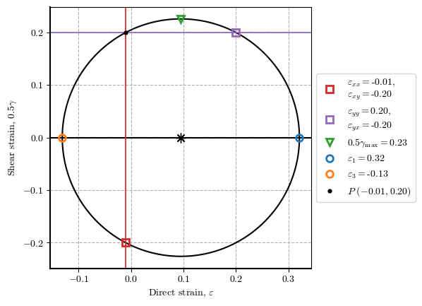
s, l = {'description_width': '60px'}, wgt.Layout(width='400px')
s_env, l_env = {'description_width': '60px'}, wgt.Layout(width='190px')
controls = {
    'ε_xx': wgt.FloatSlider(value=-0.1, min=-1, max=1, description="𝜀_xx", style=s, layout=l),
    'ε_yy': wgt.FloatSlider(value=0.2, min=-1, max=1, description="𝜀_yy", style=s, layout=l),
    'ε_xy': wgt.FloatSlider(value=-0.2, min=-1, max=1, description="𝜀_xy", style=s, layout=l),
    'plot_pole': wgt.Checkbox(value=False, description="Plot pole?", style=s, layout=l),
    'plot_plane': wgt.Checkbox(value=False, description="Plot a plane? → ", style=s_env, layout=wgt.Layout(width='180px')),
    'ω': wgt.FloatSlider(value=10, min=0, max=180, step=0.2, description="𝜔", style={'description_width': '10px'}, layout=wgt.Layout(width='220px')),
    'xlim': wgt.FloatRangeSlider(value=[-.3, .5], min=-1, max=1, step=.5, description='x-axis:', readout_format='.0f', style=s, layout=l),
    'ylim': wgt.FloatRangeSlider(value=[-.3, .3], min=-1, max=1, step=.5, description='y-axis:', readout_format='.0f', style=s, layout=l),
    'static_fig': wgt.Checkbox(value=True, description='Non-vector image (improve widget performance)', disabled=False, style=s, layout=l)
}
c_all = list(controls.values())
c_pln = [wgt.HBox(c_all[4:6])]
c = c_all[:4] + c_pln + c_all[6:]
fig = wgt.interactive_output(plot_mohr_circle, controls)
wgt.HBox((wgt.VBox(c), fig), layout=wgt.Layout(align_items='center'))
Loading...
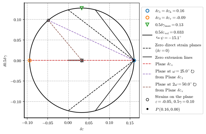
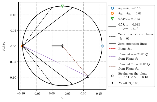
Lineas de cero extensión en el círculo de Mohr
plot_zero_ext_comp_lines(𝛿𝜀_h=-0.16, 𝛿𝜀_v=0.094, plot_plane=True, 𝜔=25)
plot_zero_ext_comp_lines(𝛿𝜀_h=0.16, 𝛿𝜀_v=-0.094, plot_plane=True, 𝜔=25)
plot_zero_ext_comp_lines(𝛿𝜀_h=-0.094, 𝛿𝜀_v=0.16, plot_plane=True, 𝜔=25)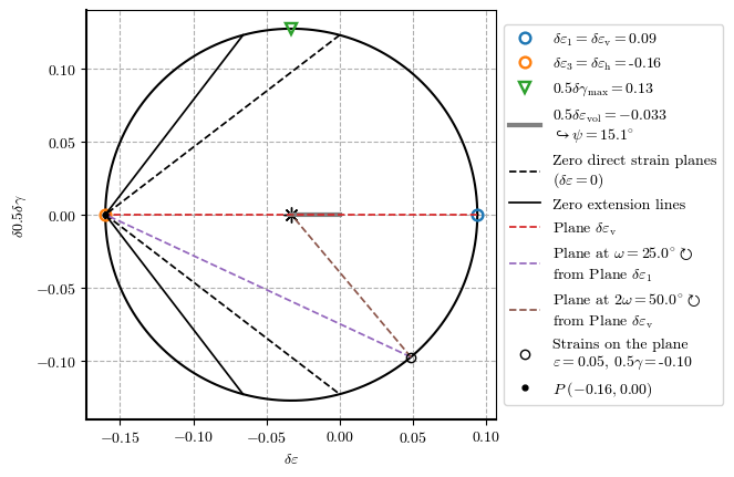
s, l = {'description_width': '60px'}, wgt.Layout(width='400px')
s_env, l_env = {'description_width': '60px'}, wgt.Layout(width='190px')
controls = {
    'δε_h': wgt.FloatSlider(value=-0.16, min=-1, max=1, step=.0001, description="𝛿𝜀_h", readout_format='.4f', style=s, layout=l),
    'δε_v': wgt.FloatSlider(value=0.0942, min=-1, max=1, step=.0001, description="𝛿𝜀_v", readout_format='.4f', style=s, layout=l),
    'plot_plane': wgt.Checkbox(value=False, description="Plot a plane? → ", style=s_env, layout=wgt.Layout(width='180px')),
    'ω': wgt.FloatSlider(value=10, min=0, max=180, step=1, description="𝜔", style={'description_width': '10px'}, layout=wgt.Layout(width='220px')),
    'xlim': wgt.FloatRangeSlider(value=[-.2, .2], min=-1, max=1, step=.02, description='x-axis:', readout_format='.2f', style=s, layout=l),
    'ylim': wgt.FloatRangeSlider(value=[-.15, .15], min=-1, max=1, step=.02, description='y-axis:', readout_format='.2f', style=s, layout=l),
    'static_fig': wgt.Checkbox(value=True, description='Non-vector image (improve widget performance)', disabled=False, style=s, layout=l)
}
c_all = list(controls.values())
c_pln = [wgt.HBox(c_all[2:4])]
c = c_all[:2] + c_pln + c_all[4:]
fig = wgt.interactive_output(plot_zero_ext_comp_lines, controls)
wgt.HBox((wgt.VBox(c), fig), layout=wgt.Layout(align_items='center'))
Loading...
- Parry, R. (2014). Mohr Circles, Stress Paths and Geotechnics (2nd ed.). CRC Press. 10.1201/9781482264982